![]()
Example: Coupled Oscillators
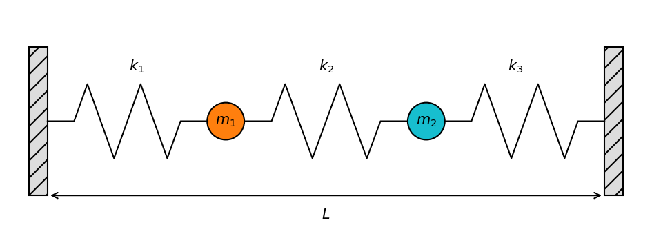
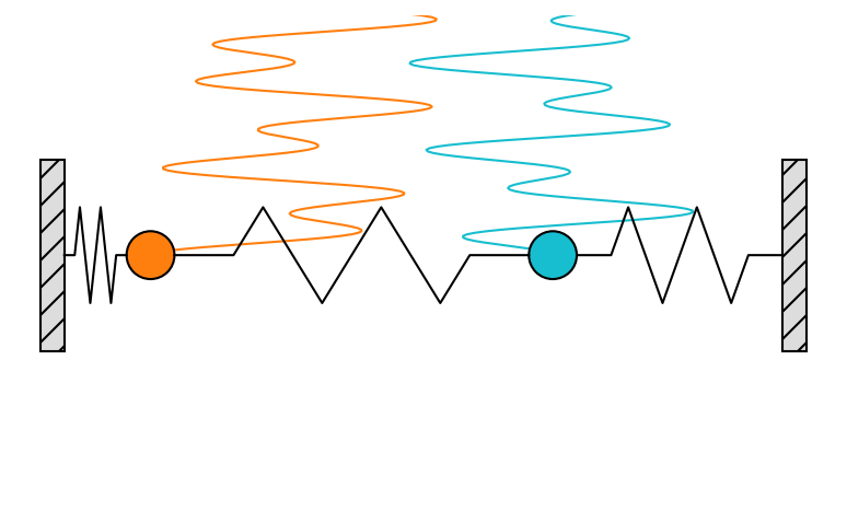
In this example we’ll have a look at coupled oscillations of two bodies with masses \(m_i\) connected via three springs to themselves and attached to walls. The goal is to calculate the time evolution of this system if it’s not in equilibrium. The springs have spring constants of \(k_i\) and lengths of \(l_i\) when no forces are acting on them. The distance between the walls is \(L\).
[1]:
k1, l1 = 10., 6.
k2, l2 = 20., 6.
k3, l3 = 10., 6.

m1, m2 = 1., 1.

L = 15.
Springs connected serially have a resulting spring constant of \(K\), which is the inverse sum of the individual spring constants.
[2]:
Kinv = 1./k1 + 1./k2 + 1./k3
K    = 1./Kinv
The force exerted by a spring is given by
\(\Large \vec{F} = -k\cdot\vec{d}\)
where \(\vec{d}\) is the displacement vector from its equilibrium position. The system can be more easily solved by solving for the time evolution of the displacements \(\vec{d}_i\) of the bodies. To convert it back into actual coordinates, we first have to finde the equilibrium positions \(\vec{x}_i\) of the bodies.
If the system is in equilibrium, the forces acting on each individual spring are identical.
[3]:
F = - ( L - ( l1 + l2 + l3 ) ) * K
From this we can calculate the equilibrium positions.
[4]:
x1 = l1 - F/k1
[5]:
x2 = F/k3 + L - l3
In equilibrium our system looks as follows.
[6]:
import matplotlib.pyplot as plt
import matplotlib.patches as patches
plt.rcParams["figure.dpi"] = 150.
import numpy as np
[7]:
def getspring(l1, l2, bw):
    l1 = float(l1)
    l2 = float(l2)
    bw = float(bw)
    L = l2 - l1
    d = L/6.
    x = np.array([l1, d, d/2., d, d, d, d/2., d], dtype=float)
    for i in range(1, 8):
        x[i] += x[i-1]
    y = np.array([0., 0., 2.*bw, -2.*bw, 2.*bw, -2*bw, 0., 0.], dtype=float)
    return x, y
[8]:
def plot_system(bw, x1, x2, L):

    fig, ax = plt.subplots()
    ax.axis("off")
    ax.set_aspect(1.)

    rectl = patches.Rectangle((-bw, -4.*bw), bw, 8.*bw, linewidth=1, edgecolor="#000000", facecolor="#dddddd", hatch="//")
    ax.add_patch(rectl)
    rectr = patches.Rectangle((L, -4.*bw), bw, 8.*bw, linewidth=1, edgecolor="#000000", facecolor="#dddddd", hatch="//")
    ax.add_patch(rectr)
    body1 = patches.Circle((x1, 0), bw, linewidth=1, edgecolor="#000000", facecolor="C1")
    ax.add_patch(body1)
    body2 = patches.Circle((x2, 0), bw, linewidth=1, edgecolor="#000000", facecolor="C9")
    ax.add_patch(body2)

    s1x, s1y = getspring(0., x1-bw, bw)
    ax.plot(s1x, s1y, c="#000000", lw=1)

    s2x, s2y = getspring(x1+bw, x2-bw, bw)
    ax.plot(s2x, s2y, c="#000000", lw=1)

    s3x, s3y = getspring(x2+bw, L, bw)
    ax.plot(s3x, s3y, c="#000000", lw=1)

    ax.set_xlim(-2.*bw, L+2.*bw)
    ax.set_ylim(-3., 3.)

    fig.tight_layout()

    return fig, ax
[9]:
bw = 0.5
fig, ax = plot_system(bw, x1, x2, L)

ax.text((x1+0.)/2., 3*bw, "$k_1$", verticalalignment="center", horizontalalignment="center")
ax.text((x2+x1)/2., 3*bw, "$k_2$", verticalalignment="center", horizontalalignment="center")
ax.text((L +x2)/2., 3*bw, "$k_3$", verticalalignment="center", horizontalalignment="center")

ax.text(x1, 0., "$m_1$", verticalalignment="center", horizontalalignment="center")
ax.text(x2, 0., "$m_2$", verticalalignment="center", horizontalalignment="center")

ax.annotate(text='', xy=(0., -4.*bw), xytext=(L, -4.*bw), arrowprops=dict(arrowstyle='<->', lw=1))
ax.text(L/2, -5.*bw, "$L$", verticalalignment="center", horizontalalignment="center")

plt.show()
We know want to displace mass \(m_1\) from its equilibrium position and calculate the time evolution of the whole system.
The force acting on \(m_1\) is given by
\(\Large F_1 = m\dot{v_1} = -(k_1 + k_2) \cdot d_1 + k_2 \cdot d_2\)
Vector notation is ommited since the problem is one-dimensional. The change in the displacement \(d_1\) is given by
\(\Large \dot{d_1} = v_1\)
Similarily for the second body
\(\Large F_2 = m\dot{v_2} = -(k_2 + k_3) \cdot d_2 + k_2 \cdot d_1\)
\(\Large \dot{d_2} = v_2\)
This is a system of coupled differential equations that can be written in matrix form
\(\Large \begin{pmatrix} \dot{d_1} \\ \dot{d_2} \\ \dot{v_1} \\ \dot{v_2} \end{pmatrix} = \begin{pmatrix} 0 & 0 & 1 & 0 \\ 0 & 0 & 0 & 1 \\ -\frac{k_1+k_2}{m_1} & \frac{k_2}{m_1} & 0 & 0 \\ \frac{k_2}{m_2} & -\frac{k_2+k_3}{m_2} & 0 & 0 \end{pmatrix} \cdot \begin{pmatrix} d_1 \\ d_2 \\ v_1 \\ v_2 \end{pmatrix}\)
or short
\(\Large \frac{\mathrm{d}}{\mathrm{d}t} \vec{Y} = \mathbf{J} \cdot \vec{Y}\)
with the state vector \(\vec{Y}\) and the Jacobian \(\mathbf{J}\).
We can now start setting up the frame.
[10]:
from simframe import Frame
[11]:
sim = Frame(description="Coupled Oscillators")
[12]:
import numpy as np
[13]:
Y = np.array([-3., 0., 0., 0.])
sim.addfield("Y", Y, description="State vector")
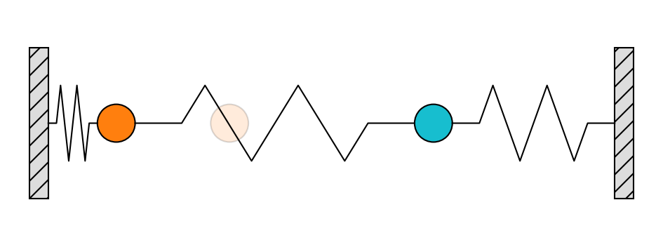
In this configuration mass \(m_1\) is displaced by \(3\) to the left while \(m_2\) is in its equilibrium position. Both bodies are at rest.
We set up the time as integration variable.
[14]:
sim.addintegrationvariable("t", 0., description="Time")
[15]:
def dt(sim):
    return 0.1
[16]:
sim.t.updater = dt
We define the snapshots according the frames per second and maximum simulation time that we want to have in the animation later.
[17]:
fps = 30.
t_max = 15.
[18]:
sim.t.snapshots = np.arange(0., t_max, 1./fps)
In principle this would be enough to run the simulation. But for convenience we set up a few more fields and groups.
[19]:
sim.addgroup("b1", description="Body 1")
sim.addgroup("b2", description="Body 2")

# Body 1
sim.b1.addfield("m" , m1, description="Mass", constant=True)
sim.b1.addfield("d" , 0., description="Displacement")
sim.b1.addfield("x" , 0., description="Position")
sim.b1.addfield("x0", x1, description="Equilibrium Position", constant=True)
sim.b1.addfield("v" , 0., description="Velocity")

# Body 2
sim.b2.addfield("m" , m2, description="Mass", constant=True)
sim.b2.addfield("d" , 0., description="Displacement")
sim.b2.addfield("x" , 0., description="Position")
sim.b2.addfield("x0", x2, description="Equilibrium Position", constant=True)
sim.b2.addfield("v" , 0., description="Velocity")
These fields need to be updated from the state vector.
[20]:
# Body 1
def update_d1(sim):
    return sim.Y[0]
sim.b1.d.updater = update_d1
def update_v1(sim):
    return  sim.Y[2]
sim.b1.v.updater = update_v1
def update_x1(sim):
    return sim.b1.x0 + sim.b1.d
sim.b1.x.updater = update_x1

# Body 2
def update_d2(sim):
    return sim.Y[1]
sim.b2.d.updater = update_d2
def update_v2(sim):
    return  sim.Y[3]
sim.b2.v.updater = update_v2
def update_x2(sim):
    return sim.b2.x0 + sim.b2.d
sim.b2.x.updater = update_x2
And we are adding more groups for the spring parameters.
[21]:
sim.addgroup("s1", description="Spring 1")
sim.addgroup("s2", description="Spring 2")
sim.addgroup("s3", description="Spring 3")

sim.s1.addfield("k", k1, description="Spring Constant", constant=True)
sim.s1.addfield("l", l1, description="Length", constant=True)
sim.s2.addfield("k", k2, description="Spring Constant", constant=True)
sim.s2.addfield("l", l2, description="Length", constant=True)
sim.s3.addfield("k", k3, description="Spring Constant", constant=True)
sim.s3.addfield("l", l3, description="Length", constant=True)
We now have to tell simframe in what order to update the fields.
[22]:
# The groups for the bodies. The order does not matter
sim.updater = ["b1", "b2"]
# The fields in the groups. Displacement has to be updated before position
sim.b1.updater = ["d", "v", "x"]
sim.b2.updater = ["d", "v", "x"]
We can now fill the fields with their initial conditions from the state vector.
[23]:
sim.update()
The initial state of the system looks as follows:
[24]:
fig, ax = plot_system(0.5, sim.b1.x, sim.b2.x, L)
circ = patches.Circle((sim.b1.x0, 0.), 0.5, linewidth=1, edgecolor="#000000", facecolor="C1", alpha=0.15)
ax.add_patch(circ)
plt.show()
Printing the complete frame structure
[25]:
sim.toc
Frame (Coupled Oscillators)
    - b1: Group (Body 1)
        - d: Field (Displacement)
        - m: Field (Mass), constant
        - v: Field (Velocity)
        - x: Field (Position)
        - x0: Field (Equilibrium Position), constant
    - b2: Group (Body 2)
        - d: Field (Displacement)
        - m: Field (Mass), constant
        - v: Field (Velocity)
        - x: Field (Position)
        - x0: Field (Equilibrium Position), constant
    - s1: Group (Spring 1)
        - k: Field (Spring Constant), constant
        - l: Field (Length), constant
    - s2: Group (Spring 2)
        - k: Field (Spring Constant), constant
        - l: Field (Length), constant
    - s3: Group (Spring 3)
        - k: Field (Spring Constant), constant
        - l: Field (Length), constant
    - t: IntVar (Time), Integration variable
    - Y: Field (State vector)
Setting up the Jacobian
For implicit schemes we have to calculate the Jacobian. Since in this case the Jacobian is constant with time, we can define it outside of the frame object.
[26]:
jac = np.array([[         0.,          0., 1., 0.],
                [         0.,          0., 0., 1.],
                [-(k1+k2)/m1,       k2/m1, 0., 0.],
                [      k2/m2, -(k2+k3)/m2, 0., 0.]], dtype=float)
[27]:
jac
[27]:
array([[  0.,   0.,   1.,   0.],
       [  0.,   0.,   0.,   1.],
       [-30.,  20.,   0.,   0.],
       [ 20., -30.,   0.,   0.]])
[28]:
def jac_impl(sim, x):
    return jac
[29]:
sim.Y.jacobinator = jac_impl
Setting up the Integrator
We can now set up the integrator just as in the previous examples.
[30]:
from simframe import Integrator
from simframe import Instruction
from simframe import schemes
[31]:
sim.integrator = Integrator(sim.t)
[32]:
sim.integrator.instructions = [Instruction(schemes.impl_1_euler_direct, sim.Y)]
Setting up the Writer
We also have to set up the writer. In this case we don’t want to write data files. So we simply write the data into a namespace
[33]:
from simframe import writers
[34]:
sim.writer = writers.namespacewriter()
sim.writer.verbosity = 0
Starting the simulation
[35]:
sim.run()
Execution time: 0:00:01
Reading data
[36]:
data = sim.writer.read.all()
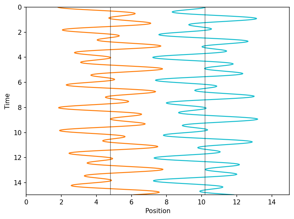
[37]:
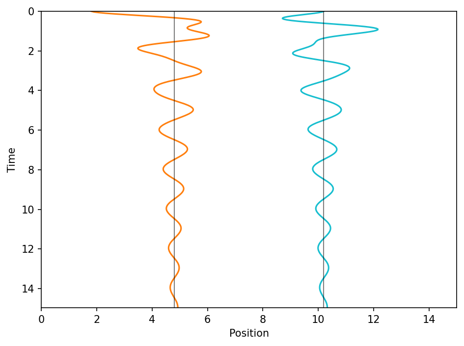
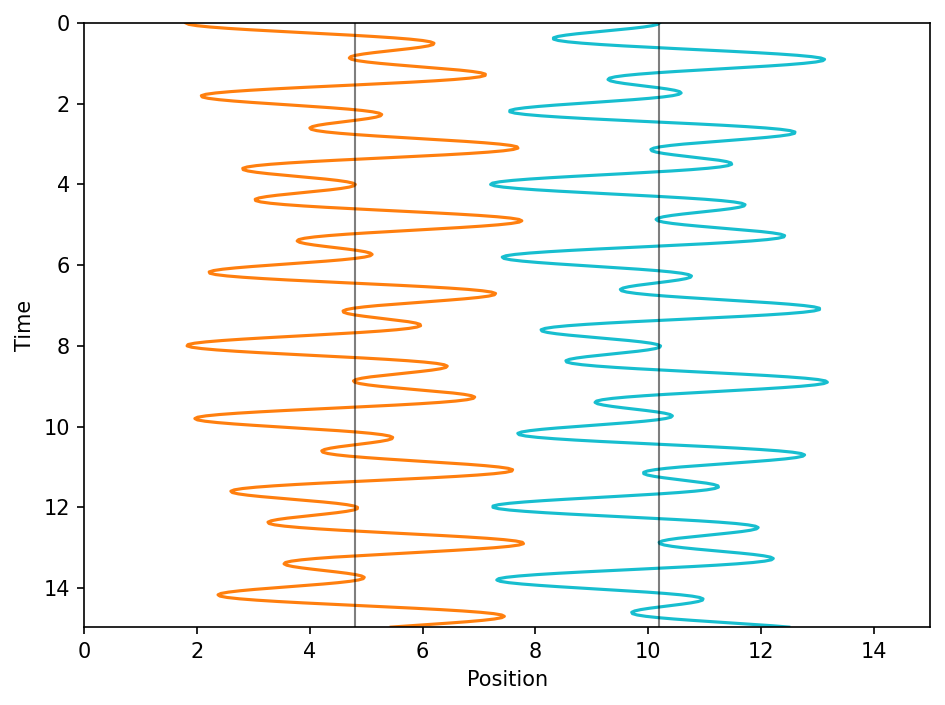
def plot_oszillations(data):
    fig, ax = plt.subplots()
    ax.plot(data.b1.x, data.t, c="C1")
    ax.plot(data.b2.x, data.t, c="C9")
    ax.axvline(data.b1.x0[0], c="#000000", alpha=0.5, lw=1)
    ax.axvline(data.b2.x0[0], c="#000000", alpha=0.5, lw=1)
    ax.set_xlim(0, L)
    ax.set_ylim(data.t[-1], data.t[0])
    ax.set_xlabel("Position")
    ax.set_ylabel("Time")
    fig.tight_layout()
    plt.show()
[38]:
plot_oszillations(data)
[39]:
from matplotlib import animation
from IPython.display import HTML
import re
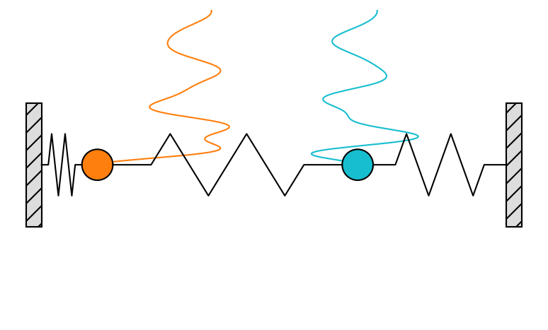
[40]:
def plot_animation(data, bw):
    fig, ax = plt.subplots()
    ax.axis("off")
    ax.set_aspect(1.)
    l1, = ax.plot(data.b1.x, data.t-data.t[0], c="C1", lw=1, zorder=-1)
    l2, = ax.plot(data.b2.x, data.t-data.t[0], c="C9", lw=1, zorder=-1)
    rectl = patches.Rectangle((-bw, -4.*bw), bw, 8.*bw, linewidth=1, edgecolor="#000000", facecolor="#dddddd", hatch="//")
    ax.add_patch(rectl)
    rectr = patches.Rectangle((L, -4.*bw), bw, 8.*bw, linewidth=1, edgecolor="#000000", facecolor="#dddddd", hatch="//")
    ax.add_patch(rectr)
    ax.set_xlim(-2.*bw, L+2.*bw)
    ax.set_ylim(-5., 5.)
    b1 = patches.Circle((data.b1.x[0], 0), bw, linewidth=1, edgecolor="#000000", facecolor="C1")
    ax.add_patch(b1)
    b2 = patches.Circle((data.b2.x[0], 0), bw, linewidth=1, edgecolor="#000000", facecolor="C9")
    ax.add_patch(b2)
    x, y = getspring(0., data.b1.x[0]-bw, bw)
    s1, = ax.plot(x, y, c="#000000", lw=1)
    x, y = getspring(data.b1.x[0]+bw, data.b2.x[0]-bw, bw)
    s2, = ax.plot(x, y, c="#000000", lw=1)
    x, y = getspring(data.b2.x[0]+bw, L, bw)
    s3, = ax.plot(x, y, c="#000000", lw=1)
    return fig, ax, l1, l2, b1, b2, s1, s2, s3
[41]:
def animate(i):
    l1.set_data(data.b1.x, data.t-data.t[i])
    l2.set_data(data.b2.x, data.t-data.t[i])
    b1.center = (data.b1.x[i], 0.)
    b2.center = (data.b2.x[i], 0.)
    x, y = getspring(0., data.b1.x[i]-bw, bw)
    s1.set_data(x, y)
    x, y = getspring(data.b1.x[i]+bw, data.b2.x[i]-bw, bw)
    s2.set_data(x, y)
    x, y = getspring(data.b2.x[i]+bw, L, bw)
    s3.set_data(x, y)
    return l1, l2, b1, b2, s1, s2, s3
[42]:
fig, ax, l1, l2, b1, b2, s1, s2, s3 = plot_animation(data, 0.5)
[43]:
anim = animation.FuncAnimation(
    fig,
    animate,
    frames=len(data.t),
    interval=1.e3/fps,
    blit=True
)
[44]:
HTML(re.sub('width="\d*" height="\d*"', 'width="100%"', anim.to_html5_video()))
[44]:
As you can see the oscillation is damped pretty quickly, which is weird because we did not include any damping term into our differential equations for the velocities.
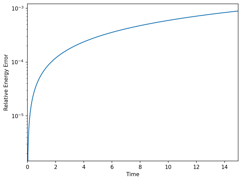
We can plot the maximum relative error of the total energy in the system.
[45]:
def plot_energy(data):
    T = 0.5*(data.b1.m*data.Y[:, 2]**2 + data.b2.m*data.Y[:, 3]**2)
    V = 0.5*(data.s1.k*data.Y[:, 0]**2 + data.s2.k*(data.Y[:, 1]-data.Y[:, 0])**2 + data.s3.k*data.Y[:, 1]**2)
    E = T + V
    dE = np.abs(E-E[0])/E[0]
    fig, ax = plt.subplots()
    ax.semilogy(data.t, dE)
    ax.set_xlabel("Time")
    ax.set_ylabel("Relative Energy Error")
    ax.set_xlim(data.t[0], data.t[-1])
    fig.tight_layout()
    plt.show()
[46]:
plot_energy(data)
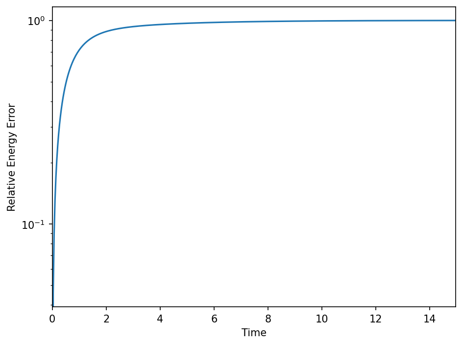
The damping is purely numerically. The cause for the damping is the implicit integrator scheme used here, that is not suited for the problem, similar to the explicit integrator used for the orbital integration.
The implicit midpoint method is simplectic, i.e., energy conserving. We can use this instead.
Resetting
[47]:
sim.Y = (-3., 0., 0., 0)
sim.update()
sim.t = 0
sim.writer.reset()
[48]:
sim.integrator.instructions = [Instruction(schemes.impl_2_midpoint_direct, sim.Y)]
[49]:
sim.run()
Execution time: 0:00:00
[50]:
data = sim.writer.read.all()
[51]:
plot_oszillations(data)
[52]:
fig, ax, l1, l2, b1, b2, s1, s2, s3 = plot_animation(data, 0.5)
[53]:
anim = animation.FuncAnimation(
    fig,
    animate,
    frames=len(data.t),
    interval=1.e3/fps,
    blit=True
)
[54]:
HTML(re.sub('width="\d*" height="\d*"', 'width="100%"', anim.to_html5_video()))
[54]:
Now the damping is gone. The energy conservation plot now reads.
[55]:
plot_energy(data)
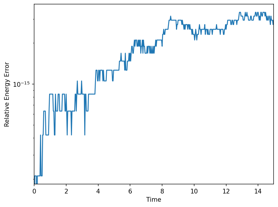
The energy error is of the order of the machine precision error.
But we could also easily use an explicit scheme. For explicit integration, we do not have to set the differentiator, since we have set a Jacobian and simframe is automatically calculating the derivative from the Jacobian.
Resetting
[56]:
sim.Y = (-3., 0., 0., 0)
sim.update()
sim.t = 0
sim.writer.reset()
[57]:
sim.integrator.instructions = [Instruction(schemes.expl_4_runge_kutta, sim.Y)]
[58]:
sim.run()
Execution time: 0:00:01
[59]:
data = sim.writer.read.all()
[60]:
plot_oszillations(data)
[61]:
fig, ax, l1, l2, b1, b2, s1, s2, s3 = plot_animation(data, 0.5)

[62]:
anim = animation.FuncAnimation(
    fig,
    animate,
    frames=len(data.t),
    interval=1.e3/fps,
    blit=True
)
[63]:
HTML(re.sub('width="\d*" height="\d*"', 'width="100%"', anim.to_html5_video()))
[63]:
[64]:
plot_energy(data)
Here the energy error larger than for the symplectic scheme, but still smaller than in the first try.