![]()
2. Advanced Integration
The equations of motion are determined by a set of two differential equations for the position \(\vec{r}\) and velocity \(\vec{v}\) of Earth and Sun..
\(\Large \frac{\mathrm{d}}{\mathrm{d}t} \vec{r} = \vec{v}\)
\(\Large m\frac{\mathrm{d}}{\mathrm{d}t} \vec{v} = \vec{F}_\mathrm{G}\)
The gravitational force \(F_\mathrm{G}\) of a body of mass \(M\) and position \(\vec{R}\) acting on a body of mass \(m\) at position \(\vec{r}\) is given by
\(\Large \vec{F}_\mathrm{G} = -GmM\frac{\vec{r}-\vec{R}}{\left| \vec{r}-\vec{R} \right|^3}\)
Creating groups
addgroup(name).[1]:
from simframe import Frame
[2]:
sim = Frame(description="Earth-Sun system")
[3]:
sim.addgroup("Sun")
sim.addgroup("Earth")
The frame object has now two groups for Earth and Sun, that can be adressed just as fields.
[4]:
sim
[4]:
Frame (Earth-Sun system)
------------------------
    Earth        : Group
    Sun          : Group
  -----
    Integrator   : not specified
    Writer       : not specified
First, we need to define a few constants.
[5]:
AU      = 1.495978707e11        # Astronomical unit [m]
day     = 8.64e4                # Day [s]
G       = 6.6743e-11            # Gravitational constant [m³/kg/s²]
year    = 3.15576e7             # Year [s]

M_earth = 5.972167867791379e24  # Mass of the Earth [kg]
M_sun   = 1.988409870698051e30  # Mass of the Sun [kg]
Creating immutable fields
[6]:
sim.Earth.addfield("M", M_earth, description="Mass [kg]")
The groups and the fields within can be easily accessed with
[7]:
sim.Earth
[7]:
Group
-----
    M            : Field (Mass [kg])
  -----
[8]:
sim.Earth.M
[8]:
5.972167867791379e+24
The mass of the Earth shall be constant throughout the simulation. We therefore set a flag so we cannot accidentally change its value.
[9]:
sim.Earth.M.constant = True
[10]:
sim.Earth
[10]:
Group
-----
    M            : Field (Mass [kg]), constant
  -----
Now we add the mass of the Sun, which we directly set to constant when adding the field.
[11]:
sim.Sun.addfield("M", M_sun, constant=True, description="Mass [kg]")
[12]:
sim.Sun
[12]:
Group
-----
    M            : Field (Mass [kg]), constant
  -----
We can do all sorts of operations with those fields, such as calculating the mass ratio.
[13]:
sim.Earth.M / sim.Sun.M
[13]:
3.0034893488507934e-06
[14]:
import numpy as np
[15]:
sim.Earth.addfield("r", np.zeros(3), description="Position [m]")
sim.Earth.addfield("v", np.zeros(3), description="Velocity [m/s]")
sim.Sun.addfield("r", np.zeros(3), description="Position [m]")
sim.Sun.addfield("v", np.zeros(3), description="Velocity [m/s]")
[16]:
sim.Earth
[16]:
Group
-----
    M            : Field (Mass [kg]), constant
    r            : Field (Position [m])
    v            : Field (Velocity [m/s])
  -----
[17]:
sim.Sun
[17]:
Group
-----
    M            : Field (Mass [kg]), constant
    r            : Field (Position [m])
    v            : Field (Velocity [m/s])
  -----
Setting the integration variable
For our simulation we need an integration variable. In our case this is the time.
[18]:
sim.addintegrationvariable("t", 0., description="Time [s]")
We’ll set the step size to a constant value of one day.
[19]:
dt = 1.*day
[20]:
def f_dt(frame):
    return dt
[21]:
sim.t.updater = f_dt
We want to integrate for two years and want to have a snapshot every ten days.
[22]:
snapwidth = 10.*day
tmax = 2.*year
[23]:
sim.t.snapshots = np.arange(0., tmax, snapwidth)
[24]:
sim
[24]:
Frame (Earth-Sun system)
------------------------
    Earth        : Group
    Sun          : Group
  -----
    t            : IntVar (Time [s]), Integration variable
  -----
    Integrator   : not specified
    Writer       : not specified
Setting the writer
As a writer we use the namespacewriter, which does not write the data into files, but stores them within a buffer in the writer.
[25]:
from simframe import writers
[26]:
sim.writer = writers.namespacewriter()
The namespacewriter is by default not writing dump files.
[27]:
sim.writer
[27]:
Writer (Temporary namespace writer)
-----------------------------------
    Data directory : data
    Dumping        : False
    Verbosity      : 1
Adding differential equations
As a next step we’ll add differential equations to the quantities. The differential equations for the positions are simple. We simply return the velocities, which we can adress with the frame argument.
[28]:
def dr_Earth(frame, x, Y):
    return frame.Earth.v

def dr_Sun(frame, x, Y):
    return frame.Sun.v
For the differential equations of the velocities we’ll write a little helper function that computes the gravitational accelleration.
[29]:
# Gravitational acceleration
def ag(M, r, R):
    direction = r-R
    distance = np.linalg.norm(direction)
    return -G * M * direction / distance**3
[30]:
def dv_Earth(frame, x, Y):
    return ag(frame.Sun.M, frame.Earth.r, frame.Sun.r)

def dv_Sun(frame, x, Y):
    return ag(frame.Earth.M, frame.Sun.r, frame.Earth.r)
Now we need to add the differential equations to their fields.
[31]:
sim.Earth.v.differentiator = dv_Earth
sim.Earth.r.differentiator = dr_Earth
sim.Sun.v.differentiator   = dv_Sun
sim.Sun.r.differentiator   = dr_Sun
Displaying the table of contents
You can also display the complete tree structure of your frame.
[32]:
sim.toc
Frame (Earth-Sun system)
    - Earth: Group
        - M: Field (Mass [kg]), constant
        - r: Field (Position [m])
        - v: Field (Velocity [m/s])
    - Sun: Group
        - M: Field (Mass [kg]), constant
        - r: Field (Position [m])
        - v: Field (Velocity [m/s])
    - t: IntVar (Time [s]), Integration variable
Inspecting memory usage
It is possible to print out the memory usage in bytes of a group with the command
[33]:
sim.memory_usage()
[33]:
317.0
Further details can be displayed with the keyword argument print_output, while skip_hidden will ommit attributes starting with underscore _:
[34]:
sim.memory_usage(print_output=True, skip_hidden=True)
    - Earth:                                   total:  56   B
        - M:                                       ()   8   B
        - r:                                     (3,)  24   B
        - v:                                     (3,)  24   B
    - Sun:                                     total:  56   B
        - M:                                       ()   8   B
        - r:                                     (3,)  24   B
        - v:                                     (3,)  24   B
    - t:                                           ()   8   B

Total: 120   B
[34]:
120.0
Iterating over group members
It is furthermore possible to iterate over the members of groups.
[35]:
for name, member in sim.Sun:
    print(name, member)
M Field (Mass [kg]), constant
r Field (Position [m])
v Field (Velocity [m/s])
This works on the Simframe object as well as for the data read in by the reader.
Setting up complex integration instructions
Next we need to set up the integrator. We integrate all quantities with the explicit Euler 1st-order scheme as in the previous tutorial, but this time he have to integrate four fields. This can be easily achieved by adding four instructions.
[36]:
from simframe import Integrator
from simframe.integration import Instruction
from simframe import schemes
[37]:
sim.integrator = Integrator(sim.t, description="Euler 1st-order")
[38]:
instructions_euler = [Instruction(schemes.expl_1_euler, sim.Earth.r),
                      Instruction(schemes.expl_1_euler, sim.Earth.v),
                      Instruction(schemes.expl_1_euler, sim.Sun.r  ),
                      Instruction(schemes.expl_1_euler, sim.Sun.v  ),
                     ]
[39]:
sim.integrator.instructions = instructions_euler
Initial conditions
Before we can start the simulation, we have to think about initial conditions.
If we simply set the Sun at rest in the center of our simulation and only set the position and velocity of the Earth, then the center of mass would have a non-zero momentum and would slowly drift away from its initial position.
So what we do first: we set the Sun’s positon to zero (i.e., don’t do anything) and the Earth’s position to a distance of 1 AU in positive x-direction. Then we’ll offset their positions to center the system on the center of mass instead onto the Sun.
[40]:
r_Earth_ini = np.array([AU, 0., 0.])
r_Sun_ini = np.zeros(3)
# Center of mass
COM_ini = (M_earth*r_Earth_ini + M_sun*r_Sun_ini) / (M_earth+M_sun)
# Offset both positions
r_Earth_ini -= COM_ini
r_Sun_ini -= COM_ini
We save them in a separate variable instead of assigning them directly for later use.
[41]:
mu = M_earth*M_sun / (M_earth+M_sun)
[42]:
v_Earth_ini = np.array([0., np.sqrt(G*M_sun/M_earth*mu/AU), 0.])
v_Sun_ini   = np.array([0., -np.sqrt(G*M_earth/M_sun*mu/AU), 0.])
Now we assign them to their fields.
[43]:
sim.Earth.r = r_Earth_ini
sim.Earth.v = v_Earth_ini
sim.Sun.r   = r_Sun_ini
sim.Sun.v   = v_Sun_ini
Starting the simulation
[44]:
sim.run()
Saving frame 0000
Saving frame 0001
Saving frame 0002
Saving frame 0003
Saving frame 0004
Saving frame 0005
Saving frame 0006
Saving frame 0007
Saving frame 0008
Saving frame 0009
Saving frame 0010
Saving frame 0011
Saving frame 0012
Saving frame 0013
Saving frame 0014
Saving frame 0015
Saving frame 0016
Saving frame 0017
Saving frame 0018
Saving frame 0019
Saving frame 0020
Saving frame 0021
Saving frame 0022
Saving frame 0023
Saving frame 0024
Saving frame 0025
Saving frame 0026
Saving frame 0027
Saving frame 0028
Saving frame 0029
Saving frame 0030
Saving frame 0031
Saving frame 0032
Saving frame 0033
Saving frame 0034
Saving frame 0035
Saving frame 0036
Saving frame 0037
Saving frame 0038
Saving frame 0039
Saving frame 0040
Saving frame 0041
Saving frame 0042
Saving frame 0043
Saving frame 0044
Saving frame 0045
Saving frame 0046
Saving frame 0047
Saving frame 0048
Saving frame 0049
Saving frame 0050
Saving frame 0051
Saving frame 0052
Saving frame 0053
Saving frame 0054
Saving frame 0055
Saving frame 0056
Saving frame 0057
Saving frame 0058
Saving frame 0059
Saving frame 0060
Saving frame 0061
Saving frame 0062
Saving frame 0063
Saving frame 0064
Saving frame 0065
Saving frame 0066
Saving frame 0067
Saving frame 0068
Saving frame 0069
Saving frame 0070
Saving frame 0071
Saving frame 0072
Saving frame 0073
Execution time: 0:00:01
Reading and plotting
Reading data from the namespace writer works identical to the writer discussed earlier.
[45]:
data_euler = sim.writer.read.all()
[46]:
import matplotlib.pyplot as plt

def plot_orbits(data):
    fig, ax = plt.subplots(dpi=150)
    ax.set_aspect(1)
    ax.axis("off")
    fig.set_facecolor("#000000")
    imax = data.t.shape[0]
    for i in range(imax):
        alpha = np.maximum(i/imax-0.1, 0.5)
        ax.plot(data.Sun.r[i, 0], data.Sun.r[i, 1], "o", c="#FFFF00", markersize=4, alpha=alpha)
        ax.plot(data.Earth.r[i, 0], data.Earth.r[i, 1], "o", c="#0000FF", markersize=1, alpha=alpha)
    ax.plot(data.Sun.r[-1, 0], data.Sun.r[-1, 1], "o", c="#FFFF00", markersize=16)
    ax.plot(data.Earth.r[-1, 0], data.Earth.r[-1, 1], "o", c="#0000FF", markersize=4)
    ax.set_xlim(-1.5*AU, 1.5*AU)
    ax.set_ylim(-1.5*AU, 1.5*AU)
    fig.tight_layout()
    plt.show()
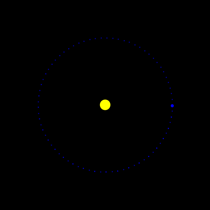
[47]:
plot_orbits(data_euler)
Leapfrog integration
As you can see, the Earth is not on a circular orbit. Its orbital distance is increasing and because of that the Earth could not achieve two full orbital cycles.
But there is a way out: Symplectic integration
In our case we first update the velocities by using half of the step size. Then we update the positions for a full time step. And finally, we update the velocities for another semi time step. We can do this by using the fstep keyword argument for the instructions, which is the fraction of the time for which this instruction is applied.
But there is one caveat: usually the fields that are integrated in an instructions set are only updated after all instructions have been executed, such that the second instruction still sees the original value of the first variable and not already the new value.
But for leapfrog integration, the instruction for the positions already need to know the new values of the velocities. And the second set of velocity instructions already need to know the new positions. We therefore have to add update instructions in between.
We do not have to add update instructions after the second set of velocity operations, because at the end of an instruction set all fields contained in the instruction set will be updated.
The new leapfrog instruction set now looks like this.
[48]:
instructions_leapfrog = [Instruction(schemes.expl_1_euler, sim.Sun.v,   fstep=0.5),
                         Instruction(schemes.expl_1_euler, sim.Earth.v, fstep=0.5),
                         Instruction(schemes.update,       sim.Sun.v             ),
                         Instruction(schemes.update,       sim.Earth.v           ),
                         Instruction(schemes.expl_1_euler, sim.Sun.r,   fstep=1.0),
                         Instruction(schemes.expl_1_euler, sim.Earth.r, fstep=1.0),
                         Instruction(schemes.update,       sim.Sun.r             ),
                         Instruction(schemes.update,       sim.Earth.r           ),
                         Instruction(schemes.expl_1_euler, sim.Sun.v,   fstep=0.5),
                         Instruction(schemes.expl_1_euler, sim.Earth.v, fstep=0.5),
                        ]
We can assign this new instruction set to our frame. To rerun the simulation we have to reset the initial conditions, that we’ve saved earlier.
[49]:
sim.integrator.instructions = instructions_leapfrog
sim.integrator.description = "Leapfrog integrator"
sim.Earth.r = r_Earth_ini
sim.Earth.v = v_Earth_ini
sim.Sun.r   = r_Sun_ini
sim.Sun.v   = v_Sun_ini
sim.t       = 0.
Additionally we have to reset the buffer of the namespace writer. Otherwise, we would simply add snapshots to the old dataset. Furthermore, we descrease the verbosity of the writer to prevent it from writing information on screen.
[50]:
sim.writer.reset()
sim.writer.verbosity = 0
[51]:
sim.run()
Execution time: 0:00:02
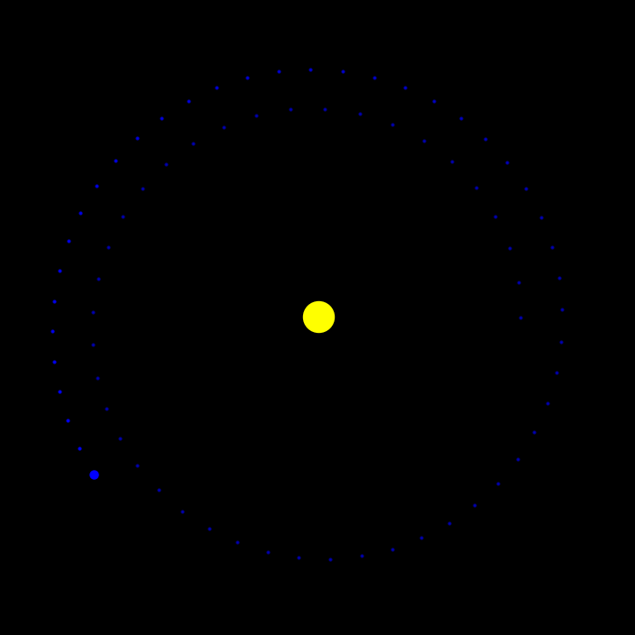
[52]:
data_leapfrog = sim.writer.read.all()
[53]:
plot_orbits(data_leapfrog)